Change Point Detection and Trend Analysis for Time Series

Ⅰ.   INTRODUCTION

Time series measurements, simulations and forecasting have important applications in various fields. The quality control and homogenization of time series must be performed prior to assessing future change and variability, or when using observations to forecast future scenarios. This is because there are many artefacts that may substantially alter the measurements, such as for wind speed: (ⅰ) station relocations, (ⅱ) anemometer height changes, (ⅲ) instrument malfunctions, (ⅳ) instruments changes, (ⅴ) different sampling intervals, and (ⅵ) observing environment changes. Therefore, advances in the quality control and homogenization procedures seek to identify and remove all artefacts in the time series so that variance in the resultant series is only driven by real changes.

Surface wind is significant for many weather events (e.g. cyclones, bushfires), ocean state climate, and viability of wind energy techniques. The characteristics of near-surface wind speed have been investigated for a variety of reasons, such as wind risk assessments, impacts of wind on soil erosion, insurance industry claims, animal welfare, climate change detection, etc. [1-8]. In addition, surface wind is a practical source of wind power generation and there is wide spread interest in surface wind for the purposes of renewable energy [9-15].

Jakob [16] discussed the challenges in developing a high-quality surface wind-speed dataset for Australia, noting issues such as changes in instrumentation (e.g. installation of Automatic Weather Stations (AWS)) and the impact of variable time zones (daylight saving). Nevertheless an up-to-date high-quality wind dataset is required for a range of research and operational activities. McVicar et al. [3] developed a gridded wind dataset for Australia, constructed using wind run data recorded at elevations below 3 m. Due to the limited and declining availability of data from anemometers at heights below 3 m [16], we recently developed improved wind datasets for Australia through: (1) inclusion of multiple sources of observed wind data (such as wind run above 3 m and daily mean wind speed at 10 m derived from hourly data), (2) consideration of local surface roughness information (mostly vegetation heights based on land cover types). The new datasets will be publicly available through SILO project [17].

The new wind datasets have been used to assess the long-term trends in wind speed over Australia in this work. Globally, there has been widespread reports of declines in measured terrestrial near-surface wind speeds [5-8, 18-20], which is contrary to the observed increase in wind speed over oceans [21, 22]. Troccoli et al. [23] reported wind speed trends in Australia are sensitive to the height of the station: they are largely negative for 2 m observations but are predominantly positive for 10 m observations. We use our new datasets to investigate these apparently contrasting wind speed trends and try to clarify the sources of such inconsistencies between 2 m wind and 10 m wind speed trends through multiple period trend analysis, change point detection, and homogenizations.

Ⅱ.   MATERIALS AND METHODS

A   Data selection

Observational data collected by the Australian Bureau of Meteorology (BoM) were used in this study. Owing to the limited availability of any single observed wind variable, we use multiple sources of data to prepare estimates of daily mean wind speed.

The number and type of instruments used by the Australian Bureau of Meteorology for recording wind data have changed significantly in recent decades. Overall, the number of stations recording 2 m wind has decreased, while the number recording wind speed at 10 m has increased substantially. These changes have been driven by the move toward fully automated stations (to reduce the cost of operation and improve reliability) at the World Meteorological Organization's agreed height of 10 m, which may also enable the data to be more easily ingested and used in global reanalysis systems.

To construct gridded datasets of the highest quality over the longest period, it is necessary to amalgamate all the available observational data. As wind speed typically increases with height in the atmospheric boundary layer, wind speeds recorded at different heights can be adjusted to a common height. Daily gridded wind speed surfaces were constructed by interpolating the available observational data using a thin plate smoothing spline with longitude, latitude, and elevation as independent variables. A two-step interpolation method [17] was used: in the first step a tri-variate spline was fitted and a generalized cross validation technique was used to identify observations which may have been erroneous, in the second step a spline was fitted to the revised dataset (with the suspect data omitted) and the surface was generated.

B   Trend analysis and change point detection

Trend analysis is defined as a process of estimating gradual change in future events from past data. Linear regressions were used to investigate trends in daily mean and annual mean wind speeds. Analyses were conducted at each grid cell using the time-series obtained by extracting data for a given pixel from the time-series of daily rasters (from 1 January 1975 to 31 December 2015). Statistical significance was assessed using the Cox-Stuart trend test.

A change point can be defined as unexpected structural changes in time series data properties such as the mean or variance. The "changepoint" R package [26] was used to identify change points. The package's "BinSeg" option was used because the Binary Segmentation method can detect multiple change points. The evaluation method was used for identifying changes in mean and variance with the following parameters: the maximum number of change points to search was set to 50 with the Schwarz Information Criterion (SIC) penalty, and the assumed test statistic was set to "Exponential".

C   Homogenization

A R package called "Climatol" [27] was employed to homogenize the wind speed time series if change points were detected for the time series. In the package change points techniques were used as a way to homogenize the time series by correcting the means for various change points (multiplication by a factor). The automatic homogenization of different wind speed time series was implemented in the recently developed Version 3.1 of the R package Climatol [27]. This approach is an advance in homogenization of climate records as it identifies change points based on monthly data, splits the daily series into homogeneous subperiods, and homogenizes them without needing the monthly corrections.

Ⅲ.   RESULTS

A   Wind speed trends

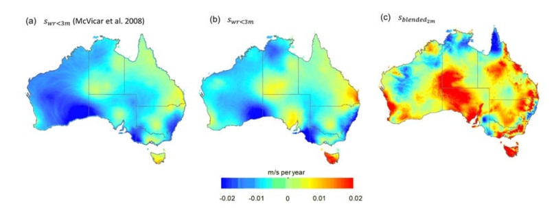
The trends in 2 m wind speed over the period 1975-2015 are shown in FIG. 1. The previously reported stilling phenomenon [3] is evident in the trend maps computed using observed wind run data below 3 m (FIG. 1(a) [3] and FIG. 1(b) (this work)). The spatially averaged trends are -0.006 m/s per year (FIG. 1(a)) and -0.005 m/s (FIG. 1(b)). The general decline in wind speed is however not evident in the trend map computed using the blended dataset ($s_{ \text{blended}_{2 \text{m}}}$, FIG. 1(c)) which shows a positive trend over most parts of Australia. The difference may be attributed to the inclusion of 10 m wind data in the $s_{ \text{blended}_{2 \text{m}}}$ datasets, and also the increasing proportion of 10 m measurements (compared to 2 m) over the base period. Given that there is wide-spread stilling reported in Ref.[8], the 10 m instrumental issue or other factors (see below) might contribute to the differences between 2 m wind speed and blended 2 m wind speed datasets.

Figure  1.  Trends in 2 m wind speeds (1975-2015) computed from datasets as follows: (a) 2 m wind only $s_{ \text{wr}<3 \text{m}}$ by McVicar et al. [3], (b) 2 m wind only $s_{ \text{wr}< \text{3 m}}$ (this work), and (c) blended 2 m wind $s_{ \text{blended}_{2 \text{m}}}$ (this work).

DownLoad: Full-Size Img PowerPoint

The time series of annual mean 2 m and 10 m wind speeds ($s_{ \text{wr}< \text{3 m}}$, $s_{ \text{wr}>3 \text{m}}$, and $s_{ \text{blended}_{2 \text{m}}}$) are shown in FIG. 2. There are statistically highly significant trends in all variables, however the trends are not consistent. There is a negative trend in 2 m wind speed $s_{ \text{wr}< \text{3 m}}$ but positive trends in 10 m wind or blended 2 m wind speed. Variability and trends in the annual wind data suggest that using a constant wind speed to estimate future wind speed or other variables such as potential evaporation is less than ideal.

Figure  2.  Annual mean 2 m and 10 m wind speeds over Australia based on datasets as follows: (a) 2 m wind only $s_{ \text{wr}<3 \text{m}}$ by McVicar et al. [3], (b) 2 m wind only $s_{ \text{wr}< \text{3 m}}$ in this work, (c) blended 2 m wind $s_{ \text{blended}_{2 \text{m}}}$ in this work, (d) 10 m wind only $s_{ \text{wr}> \text{3m}}$ (this work). Trend lines (red dotted line) are statistically significant with $p$-values as follows: (a) 3.8$\times$10$^{-5}$, (b) 2.0$\times$10$^{-5}$, (c) 2.0$\times$10$^{-5}$, (d) 2.0$\times$10$^{-4}$. Wind speed is in unit of m/s.

DownLoad: Full-Size Img PowerPoint

We hypothesise the calculated trends in near surface wind speed (negative trends at 2 m and positive trends at 10 m) are mostly due to systemic changes in data collection methods. Genuine changes in wind speed could however be caused by natural phenomena, such as abrupt phase changes in the Pacific Decadal Oscillation (PDO) [28, 29]. Two such changes occurred recently: circa 1996-1998 and 2014 [28]. We analyzed the distribution of the change points along years and found that there is a peak in 1997 for wind run below 3 m only. The possibility of abrupt changes in wind regimes can be another explanation for the differences in the 10 m and 2 m trends. While we do not discount physical processes driving changes in observed wind speeds, we propose most of the observed change is due to systematic bias in data collection. Straightforward computation of trends leads to the results shown in FIG. 1. Manual inspection of records however, indicates the trends at some stations may be influenced by changes in instrument type. For example, the apparent increase in 10 m wind speed (FIG. 2(d)) in the 1990s could be related to the installation of Automatic Weather Stations.

B   Change point detections

Change point and trend analysis methods (see section Ⅱ.B) were used to detect change points and compute trends. Trends were only computed on time series containing data for at least 120 days, and significance testing was used to determine if the wind speeds were increasing (positive trend), neutral (no significant trend) or decreasing (negative trend). The results (summarized in Table Ⅰ) reveal the impact that naïve computation can have on the interpretation of trends. There does not appear to be a substantial difference between trends in daily mean 2 m and 10 m wind speeds at those stations where change points were not detected (rows 7-9, Table Ⅰ). The proportion of stations at which wind speeds are decreasing, neutral or increasing are roughly similar for two wind variables ($s_{ \text{wr}>3 \text{m}}$ and $s_{ \text{wr}<3 \text{m}}$ with the proportion order ($P_{ \text{neutral}}$$>$$P_{ \text{decreasing}}$$>$$P_{ \text{increasing}}$)). In contrast, disparate trends are observed at stations where change points were detected, if the trend is fitted to the entire time series (i.e. neglecting the change points). In this case (rows 12-14, Table Ⅰ) the computed trends are potentially misleading, indicating: (ⅰ) decreasing wind speeds at the majority of stations reporting 2 m wind (62%, $s_{ \text{wr}<3 \text{m}}$); (ⅱ) increasing wind speeds at the majority of stations reporting 10 m wind (71%, $s_{ \text{wr}>3 \text{m}}$). The apparent contradiction can be resolved by examining the trends within the individual periods between change points (rows 15-17, Table Ⅰ). With this modification the proportion of stations at which wind speeds are decreasing, neutral or increasing are again roughly similar for the two wind variables ($s_{ \text{wr}>3 \text{m}}$ and $s_{ \text{wr}<3 \text{m}}$), with the proportion order ($P_{ \text{neutral}}$$>$$P_{ \text{decreasing}}$$>$$P_{ \text{increasing}}$).

Table  Ⅰ.  Change point analysis results. Observational 2 m wind ($s_{ \text{wr}< \text{3 m}}$), 10 m wind ($s_{ \text{wr}> \text{3 m}}$) datasets were analysed for change points. Trends were computed for each time series dataset, and where change points were detected within a given time series, trends were computed for the individual periods within the time series as well. Trends were only computed on datasets having 120 or more observations and significance was evaluated at the 95% confidence level.

 | Show Table

DownLoad: CSV

The preceding analysis showed that trends in daily mean 2 m and 10 m wind speeds are similar, with wind speeds either declining or not changing at the majority of stations if change points were considered. Our findings differ from previous reports of 2 m wind speeds decreasing and 10 m wind speeds increasing [23], because our analysis considered potential discontinuities in the observational records. We observe consistent trends in 2 m and 10 m datasets when the discontinuities are removed i.e. trends are not computed on datasets containing discontinuities as identified by change point analysis. We attribute the discontinuities most likely to instrumental changes and/or other site factors. For example, changes to instrumentation can be detected in the observational data for station 009021 (Perth Airport), shown in FIG. 3. Two change points are detected in the 2 m wind data (FIG. 3(a)), with the latter coinciding with the installation of a new anemometer in October 1997 [24]. The first change point (October 1987) does not appear to be related to instrumental changes as there is no record of any such change around that time in the station metadata. Two change points are also detected in the 10 m wind speed data averaged from hourly wind speed measurements (FIG. 3(b)), with both coinciding with the installation of new anemometers in October 1981 and June 1994 [24].

Figure  3.  Daily mean wind speeds at station 009021 (Perth Airport) computed from: (a) 2 m wind ($s_{ \text{wr}< \text{3 m}}$), (b) 10 m wind speed averaged from hourly measurements ($s_{\overline{ \text{ws}_{10 \text{m}}}}$). Blue lines represent the mean wind speed in each discrete period identified by change point analysis.

DownLoad: Full-Size Img PowerPoint

In addition to instrument changes, many other factors can affect the quality of wind datasets. Examples include: human errors (although the effect is declining with increasing automation), systematic drift due to instrument wear, ongoing changes in the environment (surface roughness) surrounding a station (either human induced such as new buildings or natural changes such as tree growth) and biased sampling (possible preferential installation of stations in high wind areas to support wind farm development). An example of what appears to be systematic human error is shown in FIG. 4. Station metadata [25] indicate wind run data were recorded at station 075086 (Wakool-Murray Irrigation) between Jan 1973 and November 2007, however data do not appear to be available between January 1986 and January 1996. The 2 m wind speed (derived from wind run) at this location appears to be systematically higher and more variable in the first period (up to December 1985) than in the second period (February 1996 onwards). Inspection of the raw data indicates measurements were not recorded on weekends and the accumulation day count was not recorded correctly in the first period. Consequently 2 m wind speeds in the first period are overestimated due to the wind run having accumulated over each weekend.

Figure  4.  Wind speed at 2 m ($s_{ \text{wr}<3 \text{m}}$) at station No.075086 (Wakool-Murray Irrigation). The accumulation flag appears to have been set incorrectly over the period January 1973-November 1985. The inset shows the effect that weekend accumulations of wind run has on the computed wind speed for the following Monday.

DownLoad: Full-Size Img PowerPoint

As noted earlier the accuracy of gridded surfaces is critically dependent on the number of stations reporting observations. As the number and type of wind observations have varied significantly over the historical period, we expect the quality of the gridded surfaces to consequently vary. The number of stations recording 2 m wind run appears to be declining, but this has been offset by the rapid increase in 10 m observations with the installation of Automatic Weather Stations. The preferential installation of stations in high wind areas has however the potential to introduce bias into products relying on a representative sampling, such as gridded surfaces and spatially-averaged trends.

C   Homogenizations

Change points techniques can be used as a way to homogenize the time series by correcting the means for various change points (multiplication by a factor). The daily wind speed data were firstly aggregated into monthly series and then the daily series was adjusted using the monthly detected change points. Here we show homogenization results for one station BROOME AIRPORT-No.03003 (daily mean wind speed at 10 m in FIG. 5(a) and wind run below 3 m in FIG. 5(b) using R package called "Climatol"). In FIG. 5 colored lines represent the candidates from homogenization, whereas black line represents the BoM observations. Since the wind speed data in the latest years are more accurate, we should use the data in red line in FIG. 5(a) and blue line in FIG. 5(b) as best candidates from homogenization. Using these homogenized data, the positive trend for 10 m wind speed and the negative trend for 2 m wind speed will be reduced substantially. For this specific station, we searched BoM meta-data and found that automatic weather station (AWS) at 10 m was installed on 27/07/1995, which might be the major reason for data discontinuities for this station (e.g. very large positive trend).

Figure  5.  (a) Homogenisation of daily mean wind speed at 10 m using wind run below 3 m as reference for one typical station BROOME AIRPORT (03003). (b) Homogenisation of wind run below 3 m using daily mean wind speed at 10 m as reference for the same station 03003. Colored lines represent the candidates from homogenization, whereas black line represents the BoM observations.

DownLoad: Full-Size Img PowerPoint

For wind run below 3 m (00300), Cox-Stuart test for trend analysis indicated it has a decreasing trend with p-value of 2$\times$e$^{-110}$. There is one change point detected in 1990s. However, from BoM record we could not find detailed instrumental change records before 1999. Therefore it is possible that there is naturally occurring change point for this station. As mentioned above, PDO might be the major reason for such types of naturally occurring change points detected.

Ⅳ.   CONCLUSION

In this work we analyzed surface wind speed trends based upon newly developed wind datasets for Australia. Wind speed trends show significant spatial variability with an overall decrease in 2 m wind speeds and overall increase in 10 m wind speeds. The trends were found to be strongly influenced by changes in instrumentation and when such factors were taken into consideration using change point analysis, significant trends were not found at most locations. From multiple period trend analysis based on change point detections, we found that neutral trend is most likely, followed by deceasing trend, and an increasing trend is less likely for most parts of Australia. Application of the homogenization approach found a reduced wind speed trends for both 2 m wind speed and 10 m wind speed, compared to raw wind speed data.

Ⅴ.   ACKNOWLEDGMENTS

Dr. Hong Zhang is extremely grateful to his supervisors, Prof. Nanquan Lou and Prof. Ke-Li Han for their invaluable advice, continuous support, and patience during his PhD study. Their immense knowledge and plentiful experience have encouraged Dr. Zhang in all the time of his Academic Research and Government Career.

This research was supported by the Queensland Government Department of Environment and Science, Australia.